This topic is about how populations fit into ecosystems, and how ecologists measure and manage them.
Populations, Communities and Ecosystems
What you need to know (from the AQA specification)
What you need to know (from the AQA specification)
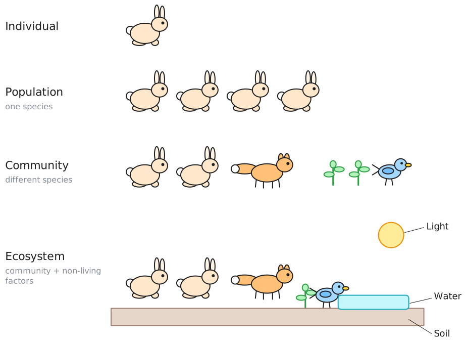
Populations of different species form a community. A community and the non-living components of its environment together form an ecosystem. Ecosystems can range in size from the very small to the very large.
Within a habitat, a species occupies a niche governed by adaptation to both abiotic and biotic conditions.
Here are some definitions to know…
- Population: A group of organisms of the same species, in a particular space, at a particular time, that can potentially interbreed (see Populations)
- Community: All the populations of different species living in the same place at the same time
- Ecosystem: A community and the non-living (abiotic) components of its environment. Ecosystems can be very small (e.g. a pond) or very large (e.g. a forest)
Habitat and niche
- Habitat: The place where an organism lives
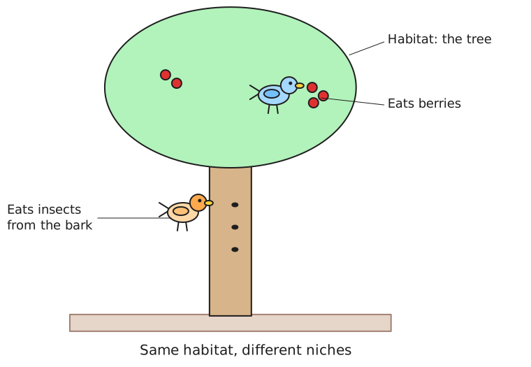
- Niche: The role of a species within its habitat, e.g. what it eats and when it’s active. No two species can occupy exactly the same niche in a habitat. A species’ niche depends on its adaptations to both:
- Abiotic conditions: the non-living factors, e.g. temperature, light, water and pH
- Biotic conditions: the living factors, e.g. food, predators and competitors
What's the difference between a habitat and a niche?
What's the difference between a habitat and a niche?
The habitat is where a species lives. The niche is its role there, e.g. what it eats, when it feeds and how it interacts with other species. So in the example above, the tree is the habitat (where both species live), and the two niches are eating insects from the bark and eating berries.
Carrying Capacity and Population Size
What you need to know (from the AQA specification)
What you need to know (from the AQA specification)
An ecosystem supports a certain size of population of a species, called the carrying capacity. This population size can vary as a result of:
- the effect of abiotic factors
- interactions between organisms: interspecific and intraspecific competition and predation.
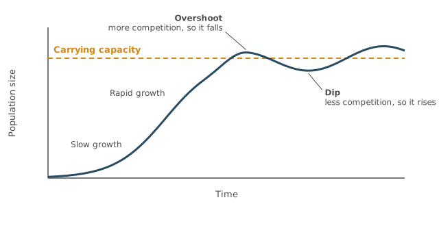
The carrying capacity is the population size of a species that an ecosystem can support in the long term, given the resources available. A population usually grows until it reaches the carrying capacity. It can then briefly overshoot, but there aren’t enough resources (e.g. food, water, shelter) to support that many individuals, so it falls back. This is why the population fluctuates around the carrying capacity.
Population size can change because of:
- Abiotic factors, e.g. if the temperature moves away from a species’ optimum (too high or too low) fewer individuals can survive and reproduce
- Biotic factors
- Interspecific competition: Competition between individuals of different species for the same resources (e.g. for food, light or shelter). The population of the less competitive species usually decreases
- Intraspecific competition: Competition between individuals of the same species. As the population grows, each individual gets fewer resources, so fewer survive and reproduce and the population falls. With less competition it rises again, so it fluctuates around the carrying capacity
- Predation: The sizes of predator and prey populations have an impact on each other (as per graph below)
Explain how intraspecific competition can cause population size to fluctuate.
Explain how intraspecific competition can cause population size to fluctuate.
- When the population is above the carrying capacity, more individuals compete for the same limited resources (e.g. food)
- Fewer individuals survive and reproduce, so the population decreases
- With fewer individuals, there is less competition and more resources for each one
- More individuals survive and reproduce, so the population increases again
Predator–prey cycles
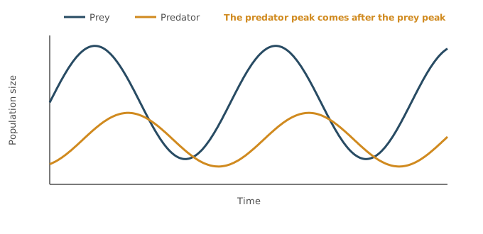
If you look at the graph above, you will notice a common pattern: the prey peak comes before the predator peak.
- When there are lots of prey, there’s more food for the predators, so the predator population increases
- More predators eat more prey, so the prey population decreases
- With less food, the predator population then decreases
- With fewer predators, the prey population increases again, and the cycle repeats
Note: In the wild, other factors (such as disease and climate) also affect both populations, so real cycles are less regular than this.
Why does the predator population peak after the prey population?
Why does the predator population peak after the prey population?
Predators need time to respond to the extra food. It takes time for more predators to survive and reproduce, so their population only increases after the prey population has increased.
Tip
Use the spec terms interspecific (between different species) and intraspecific (within one species). When you explain the effect of competition, link the resource to what it’s used for, e.g. less light means less photosynthesis, and less nitrate means fewer amino acids and proteins are made.
Growth of microorganisms
What you need to know (from the AQA specification)
What you need to know (from the AQA specification)
Students could use turbidity measurements to investigate the growth rate of a broth culture of microorganisms.
Students could use a logarithmic scale in representing the growth of a population of microorganisms.
A population of microorganisms in a broth culture follows the same pattern as any other population. It grows slowly at first, then rapidly, then levels off when nutrients run out and waste products (such as ethanol from yeast) build up.
You can follow the growth by measuring the turbidity (cloudiness) of the broth with a colorimeter. The more cells there are, the cloudier the broth, so the less light passes through.
Why use a log scale?
- In ideal conditions each cell divides, so the number of cells doubles each generation (e.g. 100, 200, 400, 800…) and quickly reaches millions
- On a normal scale, the early numbers are so small compared with the later ones that they look like zero
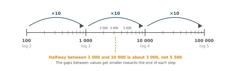
- On a log scale, each step up the axis is ×10 (100, 1000, 10 000…). The whole large range of numbers fits on one graph, and steady exponential growth shows as a straight line
How to read a log scale?
- Each labelled step is 10 times bigger than the one below (100, 1000, 10 000…).
- Sometimes the axis shows log values (2, 3, 4…) instead of the numbers.
- A log value of 3 means 103 = 1000 cells, and 4 means 10 000 cells.
- Each +1 on the log value is ×10 cells
- The space between two labels isn’t evenly split.
- Halfway between 1000 and 10 000 is about 3000, not 5500.
- To get an exact value from a log value, convert it with 10x
What the shape tells you?
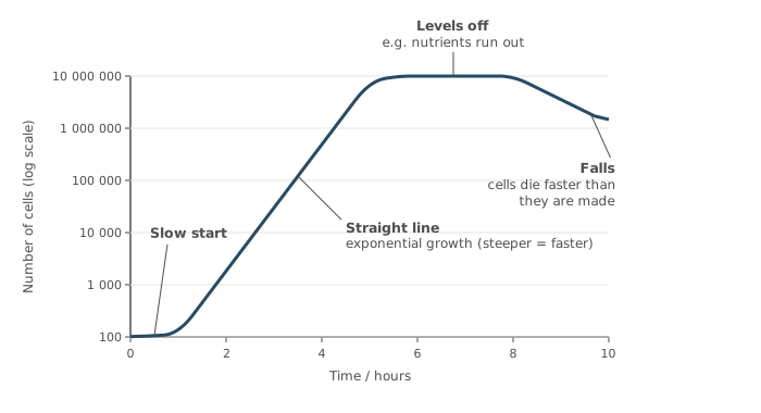
- At first the line is nearly flat (slow start) because the cells are adjusting to their new conditions (e.g. making enzymes) before they start dividing quickly. This is the lag phase
- Exponential growth means the population grows by the same factor in each time period, e.g. it doubles every 20 minutes. Every new cell divides too, so the bigger the population gets, the faster it grows
- On a log scale, growing by the same factor each time gives a straight line. A steeper line means faster growth (a shorter doubling time)
- When the line levels off, the population has stopped growing, e.g. because nutrients have run out
- If the line falls, cells are dying faster than new ones are being made
Worked example: reading a log graph and calculating a percentage increase
The graph shows the growth of a population of bacteria. Calculate the percentage increase in the number of bacteria between 1.5 hours and 2.5 hours.
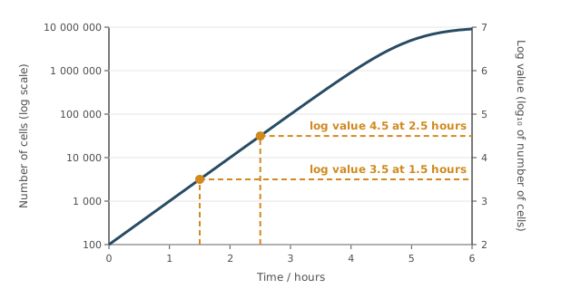
- Read the log values off the graph. Draw a line up from 1.5 hours to the curve, then across to the right-hand axis. This gives a log value of 3.5. Do the same from 2.5 hours. This gives a log value of 4.5
- Convert each log value back to a number using the 10x button on your calculator (often SHIFT then log)
- At 1.5 hours: 103.5 = 3162.3 bacteria
- At 2.5 hours: 104.5 = 31 622.8 bacteria
- Find the increase: 31 622.8 − 3162.3 = 28 460.5
- Divide by the starting number and multiply by 100: 28 460.5 ÷ 3162.3 × 100 = 900%
Exam practice
Try the 2025 exam question Percentage increase from log values in Exam Question Practice below. It uses exactly this method.
Common mistakes
- To explain why a log scale is used, refer to the large range of numbers. “The numbers are large” or “to fit on the scale” isn’t enough
- Convert log values back with 10x before you calculate anything. Working out the percentage change of the log values themselves, e.g. (5.0 − 3.0) ÷ 3.0 × 100 = 67%, is wrong
Estimating Population Size
What you need to know (from the AQA specification)
What you need to know (from the AQA specification)
The size of a population can be estimated using:
- randomly placed quadrats, or quadrats along a belt transect, for slow-moving or non-motile organisms
- the mark-release-recapture method for motile organisms. The assumptions made when using the mark-release-recapture method.
Students should be able to:
- use given data to calculate the size of a population estimated using the mark-release-recapture method.
Students could use the mark-release-recapture method to investigate the abundance of a motile species.
Counting every individual is usually impossible, so ecologists count a sample and use it to estimate the whole population. The method depends on whether the organisms move:
- Non-motile (i.e. don’t move) or slow-moving organisms (e.g. plants): randomly placed quadrats or quadrats along belt transect
- Motile (moving) organisms (e.g. insects, fish, mammals): mark-release-recapture
Non motile organisms
Measuring abundance in a quadrat
You can measure the abundance of a species in a quadrat in different ways:
- Frequency (counting):
- Count how many individuals of the species are in the quadrat, e.g. 6 daisies.
- Counting individuals is what you use to estimate population size with random quadrats, because you can find the mean and scale up
- Percentage cover:
- Estimate how much of the quadrat’s area the species covers, e.g. grass covers about half the quadrat, so 50%.
- Use it for plants where you can’t tell individuals apart, such as grasses and mosses
Random quadrats
- Divide the area into a grid, e.g. using two tape measures laid at right angles
- Use a random number generator to pick coordinates (or a way to generate a random number so there isn’t any bias in selection)
- Place a quadrat at each coordinate and count the number of individuals of the species
- Repeat for a large sample (e.g. 10 or more quadrats) and calculate the mean number per quadrat
- Estimate the total:
- First work out how many quadrats would fit in the whole site: area of the whole site ÷ area of one quadrat
- Then total = mean number per quadrat × number of quadrats that would fit
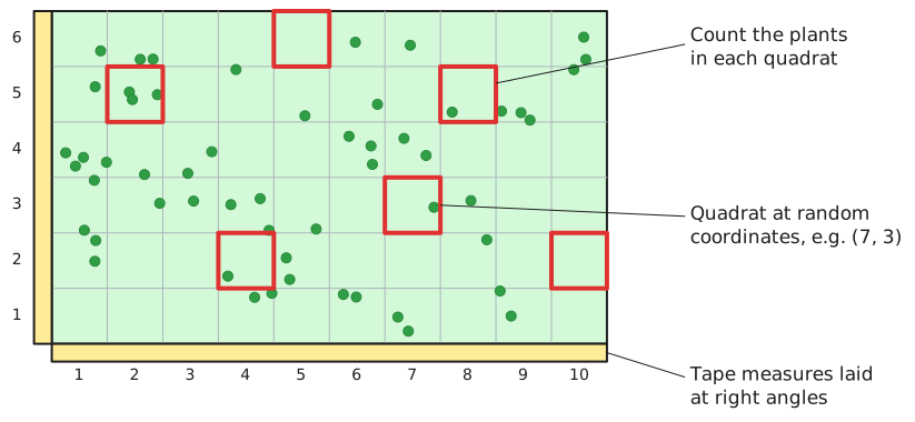
Placing quadrats at random avoids bias, e.g. choosing the spots where the plants look most common.
Worked example: estimating the number of plants in a field
A field is 100 m × 50 m. A student places 20 random quadrats, each 0.5 m × 0.5 m, and finds a mean of 3 plants per quadrat.
- Area of the field = 100 × 50 = 5000 m²
- Area of one quadrat = 0.5 × 0.5 = 0.25 m²
- Number of quadrats that would fit in the field = 5000 ÷ 0.25 = 20 000
- Estimated population = 3 × 20 000 = 60 000 plants
Tip
In a “describe how you would estimate” answer, give each step: a grid and a random number generator for coordinates (don’t throw the quadrats), a large sample, the mean per quadrat, and how you’d calculate the total. “Scale up” on its own isn’t enough.
Belt transects
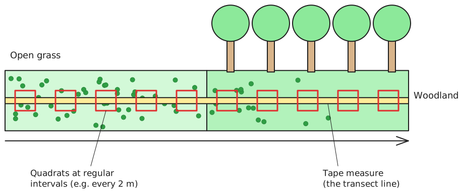
Use a belt transect when conditions change across an area, e.g. from the edge of a pond to dry land, or from open grass into woodland.
- Lay a tape measure (the transect line) across the area
- Place quadrats at regular intervals along it (e.g. every 2 m but decide distance based on what size of area you want to investigate)
- Record the abundance of the species in each quadrat, and measure the abiotic factor you’re interested in at each point (e.g. light intensity)
This shows how the distribution of a species changes along the transect.
Motile organisms
Mark-release-recapture
- Capture a sample of the population, count them and mark them (e.g. with a spot of paint, as in the picture below)
- Release them back where they were caught
- Leave enough time for them to mix back into the population
- Capture a second sample. Count the total number caught, and how many of these are marked
- Estimate the population size:
Population size = (number in first sample × number in second sample) ÷ number marked in second sample
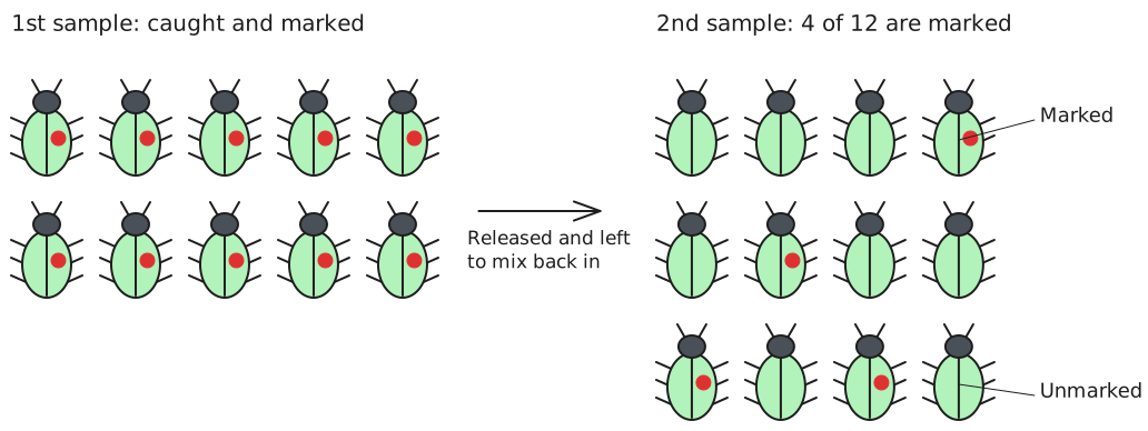
Worked example: mark-release-recapture
Ecologists catch and mark 10 beetles, then release them. A week later, they catch 12 beetles, and 4 of these are marked (as in the picture above).
Population size = (10 × 12) ÷ 4 = 30 beetles
This works because 4 out of 12 beetles in the second sample are marked (1 in 3). So the 10 marked beetles are about 1 in 3 of the whole population, and 10 × 3 = 30.
Quick sense check
- If most of the beetles in the second sample were marked, the ecologists must have caught most of the population the first time, so the population is small
- If hardly any were marked, the 10 marked beetles are spread through a much bigger crowd, so the population is large
Assumptions for mark recapture release
The formula assumes the proportion of marked individuals in the second sample is the same as in the whole population. This relies on these assumptions being true:
- The marked individuals mix evenly back into the population
- The mark doesn’t affect survival, e.g. it isn’t toxic and doesn’t make the animal easier for predators to see
- The mark isn’t lost (e.g. doesn’t rub or wash off) between the samples
- There are no births, deaths, immigration or emigration between the two samples
Common mistakes
- The second sample is the total caught the second time (marked + unmarked), not just the unmarked ones
- Divide by the number of marked individuals in the second sample (e.g. the 4 marked beetles), not the unmarked ones
A population is estimated at 600. In the first sample, 60 were marked. The second sample contained 50 individuals. How many of the second sample were marked?
A population is estimated at 600. In the first sample, 60 were marked. The second sample contained 50 individuals. How many of the second sample were marked?
Rearrange the equation: number marked in second sample = (first sample × second sample) ÷ population size
= (60 × 50) ÷ 600 = 5
Why might mark-release-recapture give an unreliable estimate in a very large lake?
Why might mark-release-recapture give an unreliable estimate in a very large lake?
Either of these:
- The marked fish are unlikely to spread out evenly through such a large lake, e.g. they may stay in one area
- You’re less likely to recapture the marked fish
Make sure your answer is about the lake being large. Marks washing off, or births and deaths, could happen in any lake, so they don’t answer the question.
Succession
What you need to know (from the AQA specification)
What you need to know (from the AQA specification)
Ecosystems are dynamic systems.
Primary succession, from colonisation by pioneer species to climax community.
At each stage in succession, certain species may be recognised which change the environment so that it becomes more suitable for other species with different adaptations. The new species may change the environment in such a way that it becomes less suitable for the previous species.
Changes that organisms produce in their abiotic environment can result in a less hostile environment and change biodiversity.
Ecosystems are dynamic, which means they change over time (often hundreds of years).
Definition
Succession is the gradual change in the species in a community over time.
Primary succession starts on land where there is no soil, e.g. bare rock after a volcanic eruption, or newly formed sand dunes.
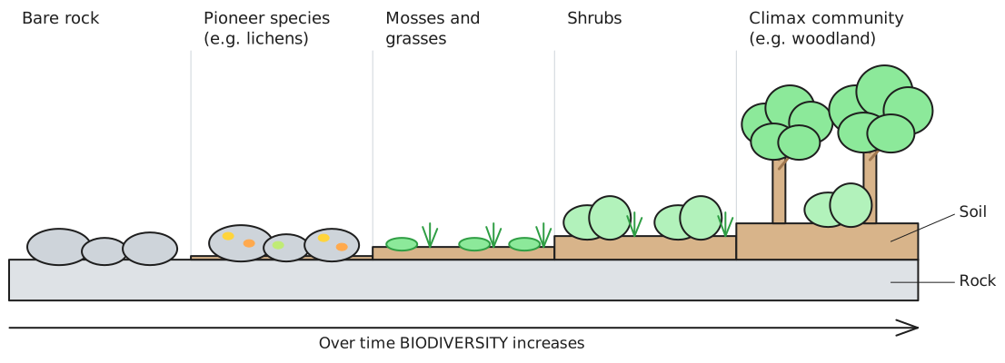
- Pioneer species colonise the bare ground (e.g. lichens on rock). They are adapted to the hostile conditions, such as little water and few nutrients
- The pioneer species change the abiotic environment, e.g. when they die and decompose, they form a thin layer of soil that holds water and nutrients
- The environment becomes less hostile, so new species with different adaptations can colonise (e.g. mosses and grasses, then shrubs)
- The new species may change the environment so that it becomes less suitable for the previous species, which are outcompeted
- As the environment becomes less hostile (e.g. soil, grasses, shrub), biodiversity increases
- Eventually a stable climax community forms (e.g. woodland)
Secondary succession happens where soil is already present, e.g. after a forest fire or when farmland is abandoned. It’s faster, because it doesn’t have to start from bare ground.
Why does biodiversity usually increase during succession?
Why does biodiversity usually increase during succession?
As the environment becomes less hostile (deeper soil, more water and nutrients), more species can survive there. More plant species provide more food sources and habitats, so more animal species can live there too.
Tip
In a “describe and explain succession” answer:
- Start with pioneer species colonising the bare ground
- Be specific about how each stage changes the environment, e.g. pioneer species die and decompose to form soil
- Say this makes the environment less hostile or more suitable for new species
- Finish with the increase in biodiversity and the climax community
- Say “species”, not “organisms” or “plants”, and don’t describe natural selection instead
Conservation and Managing Succession
What you need to know (from the AQA specification)
What you need to know (from the AQA specification)
Conservation of habitats frequently involves management of succession.
Students should be able to:
- show understanding of the need to manage the conflict between human needs and conservation in order to maintain the sustainability of natural resources
- evaluate evidence and data concerning issues relating to the conservation of species and habitats and consider conflicting evidence
Some habitats, such as heathland and grassland, are not climax communities. If succession were left to carry on, they would turn into woodland and certain species that depend on heathland and grassland would be lost. So conservation often means managing succession to stop it reaching the climax community.
Examples of conservation activities:
- Grazing: animals such as sheep eat the young shoots of shrubs and trees, so they can’t take over
- Managed burning: clears woody plants, and the habitat plants (e.g. heather) grow back first
- Mowing or cutting: stops shrubs and trees establishing
There is often a conflict between human needs and conservation, e.g. land is needed for farming, housing and timber, but this destroys habitats. Sustainable approaches try to meet human needs without using up natural resources, e.g. replanting trees after felling, or fishing quotas.
In the exam, you may be asked to evaluate data about a conservation issue. Use the data, consider evidence on both sides, and look at how reliable it is (e.g. sample size, and whether a correlation really shows a cause).
Why might conservationists let sheep graze on a heathland?
Why might conservationists let sheep graze on a heathland?
To manage succession. The sheep eat the young shoots of shrubs and trees, which stops the heathland turning into woodland, so the heathland habitat and the species that depend on it are conserved.
Required Practical 12: Distribution of a Species
What you need to know (from the AQA specification)
What you need to know (from the AQA specification)
Required practical 12: Investigation into the effect of a named environmental factor on the distribution of a given species.
Students could:
- investigate the distribution of organisms in a named habitat using randomly placed frame quadrats, or a belt transect
- use both percentage cover and frequency as measures of abundance of a sessile species.
Example: the effect of light intensity on the distribution of a plant, from open grass into woodland
- Lay a belt transect from the open grass into the woodland
- Place a quadrat at regular intervals along the transect (e.g. every 2 m)
- In each quadrat, record the abundance of the plant as percentage cover or frequency
- At each quadrat, measure the light intensity with a light meter
- Keep other variables as similar as possible, e.g. take all readings at the same time of day, and have the same person estimate percentage cover each time
- Plot abundance against light intensity, and use a statistical test (e.g. a correlation coefficient) to see if there’s a significant relationship
Why would you use percentage cover rather than counting individual plants?
Why would you use percentage cover rather than counting individual plants?
Some plants, such as grasses and mosses, grow in clumps or mats, so it’s very hard to tell where one individual ends and the next begins. Percentage cover is quicker and more practical for these species.
How this topic is tested
This analysis is based on past paper data from 2017 to 2025. It is intended for interest only and is not predictive of what will appear in future papers.
- Tested in 9 of 9 years (2017–2025): 44 question parts worth 113 marks.
- 2nd most-examined topic overall by marks, 1st in Unit 7.
Marks by year
Most-tested spec points
- Estimating Population Size: tested in 13 parts (36 marks)
- Succession: tested in 7 parts (19 marks)
- Carrying Capacity, Competition & Predation: tested in 8 parts (13 marks)
- Conservation & Managing Succession: tested in 3 parts (7 marks)
- Communities, Ecosystems & Niches: tested in 2 parts (5 marks)
- Mark-Release-Recapture in Practice: tested in 1 part (3 marks)
Also links to: Explaining Selection, Drift & Speciation, Species & Courtship Behaviour, Reproductive Separation & Speciation.
Maths and practical skills
- Using equations (MS 2.2, 2.3): e.g. 2025 P3 Q3.3
- Logarithms and log scales (MS 2.5): e.g. 2025 P3 Q1.2
- Sampling in fieldwork (AT k): e.g. 2019 P2 Q9.1
- Percentages, ratios and fractions (MS 0.3): e.g. 2025 P3 Q1.2
- Aseptic technique (AT i): e.g. 2018 P3 Q6.6
- Units and standard form (MS 0.1): e.g. 2024 P2 Q5.3
- Standard deviation and range (MS 1.10): e.g. 2024 P3 Q6.7
- Choosing and using a statistical test (MS 1.9): e.g. 2021 P2 Q9.3
Exam Question Practice
Past paper questions on this topic. Try each one before opening the answer.
In potato plant fields, fat hen plants can grow up to a height of 2 m and absorb large quantities of nutrients from the soil.
Fat hen has a negative effect on the growth of potato plants.
Use the information provided to explain why.
In your answer, name the type of competition occurring between fat hen plants and potato plants.
(3 marks)
Hint
What type of competition is it between different species? What resources might plants compete for? Link each resource to specific biological molecules.
Mark Scheme
- Interspecific (competition) (1 mark)
- Less/no light (for potato plant) so less/no photosynthesis (1 mark)
- Less nitrates/nitrogen to produce amino acids/protein/DNA/RNA/ATP
OR Less phosphate/phosphorus to produce DNA/RNA/phospholipids/RuBP/GP/triose phosphate/NADP/ATP (1 mark)
Comments from mark scheme
Tips from examiner reports
Tips from the examiner report
- Name the competition: interspecific (between different species), not intraspecific
- Link less light to less photosynthesis, not just “less growth”
- Link nutrients to what they make: less nitrate for amino acids, proteins or DNA; less phosphate for DNA, ATP or phospholipids
A weed is a plant growing where it is not wanted. Fat hen is a weed which grows in some crop fields.
Describe how you could estimate the number of fat hen plants in a field.
(5 marks)
Hint
Describe: grid setup, random sampling method, what to count, sample size for reliability. How do you scale up from quadrat to whole field?
Mark Scheme
- Use a grid
OR Divide field/area into squares (1 mark) - Method of obtaining random coordinates/numbers e.g. calculator/computer/random numbers table/generator (1 mark)
- Count number/frequency in a quadrat (1 mark)
- Large sample and calculate mean number (per quadrat) (1 mark)
- Multiply mean number of plants per m² by area of field
OR Divide area of field by area of quadrat x mean number of plants per quadrat
OR Multiply mean number of plants per quadrat/section by number of quadrats/sections in field (1 mark)
Comments from mark scheme
1. Accept use of tape measures/map/area with coordinates.
1. Accept Belt transect.
2. If transect method used accept quadrats at regular intervals.
3. Ignore amount/abundance.
3, 4 and 5. Accept sections/squares for quadrats.
4 and 5. Accept ‘average’ for ‘mean’.
4. Accept large sample and method of calculating mean.
4. Accept many/multiple for large sample but ignore several.
4. If a specific number is given it must be 10 or more.
5. Do not allow ‘scale up’ without further qualification.
Tips from examiner reports
Tips from the examiner report
- Use a grid and random coordinates (e.g. a random number generator); don’t “throw quadrats”
- Count the number of fat hen plants in each quadrat, in a large sample (10 or more), and calculate the mean
- Explain how to get the total: area of field ÷ area of quadrat × mean number per quadrat. “Scale up” on its own isn’t enough
What earned marks
- A grid and random coordinates were well known
Ecologists investigated the population size of C. graminis using the mark-release-recapture method.
Table 2 shows the ecologists’ results.
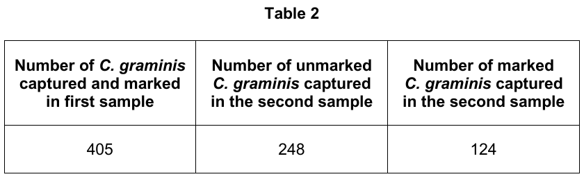
Use the data provided in Table 2 to estimate the population size of C. graminis.
Show your working.
Answer = ________ beetles
(2 marks)
Hint
The second sample is the marked plus the unmarked beetles. Population = number marked in first sample × total in second sample ÷ number marked in second sample.
Mark Scheme
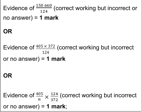
- Correct answer of 1215 (2 marks)
For 1 mark:
Evidence of 810 (not calculated total number in 2nd sample) = 1 mark
OR Evidence of 608 (divided by unmarked rather than marked) = 1 mark
OR
Tips from examiner reports
Tips from the examiner report
- The total in the second sample is marked + unmarked (248 + 124 = 372); using only 248 gave the wrong answer of 810
- Divide by the number of marked beetles recaptured (124), not by the unmarked beetles
- Population = 405 × 372 ÷ 124 = 1215
Succession occurs in natural ecosystems.
Describe and explain how succession occurs.
(4 marks)
Hint
Which species colonise first, and what do they do to the environment? How does that let other species in, and where does succession end?
Mark Scheme
Max 4 marks
- (Colonisation by) pioneer species (1 mark)
- Pioneers/species/organisms change the environment/habitat/conditions/factors (1 mark)
- (Environment becomes) less hostile for other/new species
OR (Environment becomes) more suitable for other/new species
OR (Environment becomes) less suitable for previous species (1 mark) - Change/increase in diversity/biodiversity (1 mark)
- (To) climax community (1 mark)
Comments from mark scheme
2. Accept example of change e.g. forms soil/humus/organic matter/nutrients.
2. Must convey idea of change being caused by pioneers/species/organisms
3. Accept previous species out-competed.
4. Ignore increase in genetic diversity.
Tips from examiner reports
Tips from the examiner report
- Use precise terms: ‘species’, not ‘organism’ or ‘plant’; ‘more suitable’ or ‘less hostile’, not ‘more hospitable’ or ‘more habitable’
- Include the change (increase) in biodiversity during succession, which few students mentioned
- Don’t describe natural selection or speciation instead
Figure 4 shows a typical population growth curve for yeast under laboratory conditions.
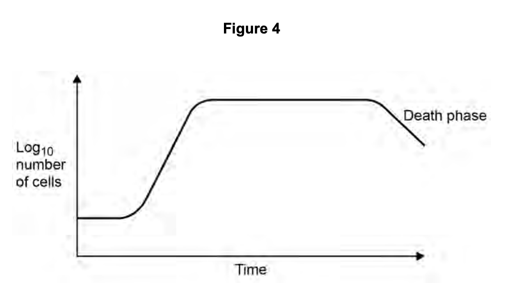
Explain why a log scale is used to record the number of cells.
(1 marks)
Hint
How much does the number of yeast cells change between the start and the peak? Why would an ordinary scale struggle to show that?
Mark Scheme
Large range/difference/increase in numbers (1 mark)
Comments from mark scheme
1. Accept reference to exponential (increase)
1. Ignore if the answer only refers to numbers being high
I. Ignore to ‘fit on the scale’
Tips from examiner reports
Tips from the examiner report
- Refer to the range: the numbers increase over a very large range (exponentially); ‘the numbers are large’, ‘to fit on the scale’ or ‘more accurate’ isn’t enough
Microbiologists investigated the effect of two temperatures on the population growth of a species of bacterium.
They grew separate bacterial cultures in identical nutrient media at 20 °C and 24 °C for 8 hours.
Figure 1 shows the estimated final population size of each culture.
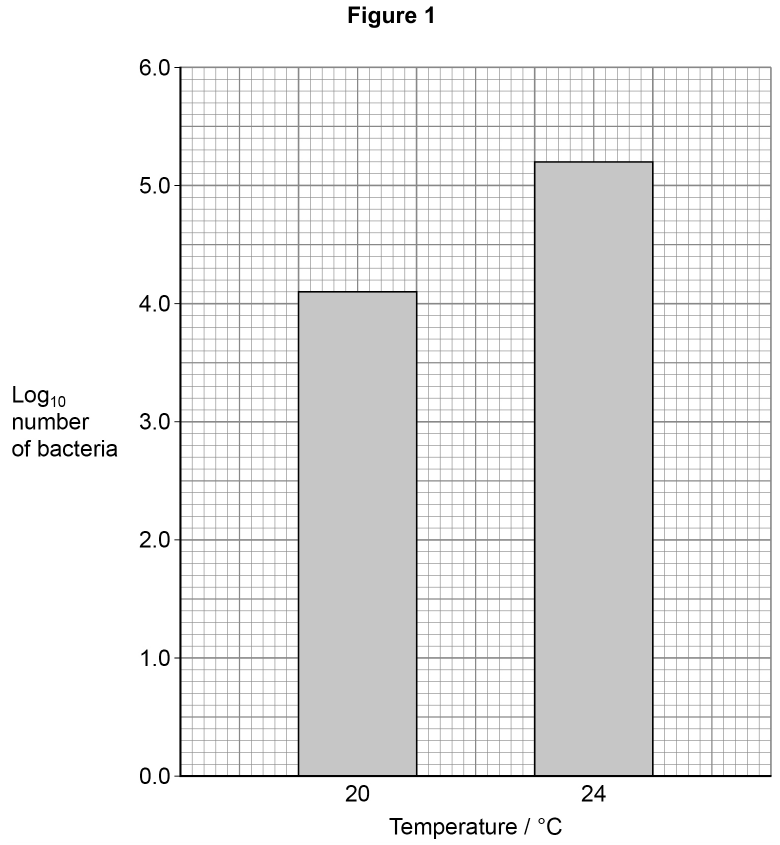
The bacterial population at 24 °C is larger than that at 20 °C
Calculate this difference as a percentage increase.
The actual number of bacteria can be calculated from the log₁₀ value by using the 10ˣ button on your calculator.
Give your answer to the nearest whole number.
Show your working.
Percentage increase = ________
(2 marks)
Hint
Convert each log value into an actual number using the 10ˣ button first. Then percentage increase = (new – original) ÷ original × 100.
Mark Scheme
Walkthrough
Step 1: read the log values from Figure 1. The population is 4.1 at 20 °C and 5.2 at 24 °C (log₁₀ values).
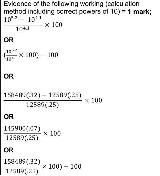
Step 2: convert each log value with the 10x button. 104.1 = 12 589.3 bacteria at 20 °C and 105.2 = 158 489.3 bacteria at 24 °C.
Step 3: find the increase. 158 489.3 − 12 589.3 = 145 900.1
Step 4: divide by the original number and multiply by 100. 145 900.1 ÷ 12 589.3 × 100 = 1158.9, so 1159% to the nearest whole number.
Mark scheme
- Correct answer of 1159 (2 marks)
For 1 mark:
Evidence of 1158 (incorrect rounding) = 1 mark
OR Evidence of 1158 followed by any number of decimal places (not to nearest whole number) = 1 mark
OR Evidence of 1259 (answer that failed to subtract 100) = 1 mark
OR Evidence of 12 (not multiplied by 100) = 1 mark
OR Evidence of 145 900(.0651) (calculation of increase in number of bacteria) = 1 mark
OR Evidence of 92 (dividing by 105.2 instead of 104.1) = 1 mark
OR Evidence of 27 (percentage increase of log values read from graph) = 1 mark
OR
Tips from examiner reports
Tips from the examiner report
- Convert the log values first, using the 10ˣ button (not the log button): 10^5.2 and 10^4.1
- Don’t find the percentage increase of the log values themselves; that gave the wrong answer of 27
- Percentage increase = (difference ÷ original) × 100, rounded to the nearest whole number: 1159
3. Accept any named organic nitrogen or phosphorus containing molecule.